hpdz.net
High-Precision Deep Zoom
Still Image Galleries
Introduction
While I love animations, you can't hang one on your wall. In addition, due limits on time and computing resources, animations generally can't be rendered to the same high quality as a single still image. Some of the images on this page are in super-high resolution and are drawn with very aggressive supersampled pixel averaging for anti-aliasing to produce picture-perfect results, suitable for framing.
Several galleries show images of various types of fractals.
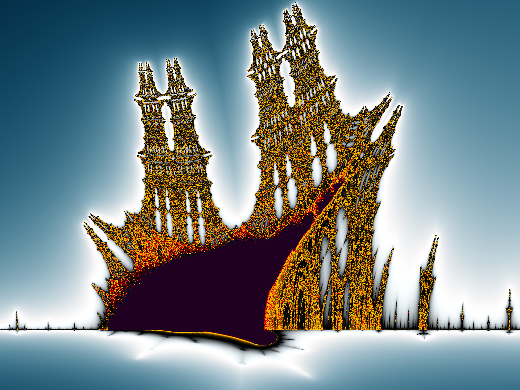
- Burning Ship Fractal
- Mandelbrot Set
- Cubic Mandelbrot Set
- Nova Fractal
- Phoenix Fractal (Henon)
- Newton and Halley Fractals
- Secant Method Fractals
- Bat Fractal
- Magnet Fractal
Click on a link to go the gallery, or scroll down to see examples from each gallery.
Julia Set Maps
Several large Julia set maps are here for various fractal types.
Other Images
Check out the bloopers section too. These are images caused by software bugs. Nobody's perfect, and these are proof that I'm no excpetion. I'm sure this section will continue to grow.
Finally, three images especially nice images that were submitted to the Fractal Forums 2009 2D Image Contest. One of them placed third. Unfortunately, HPDZ had to pass on the 2010 contest due to lack of time but will be back in 2011.
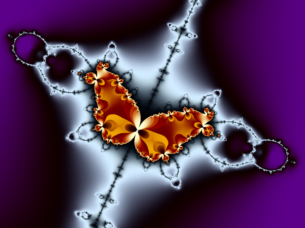 Secant Butterfly Third Place! | 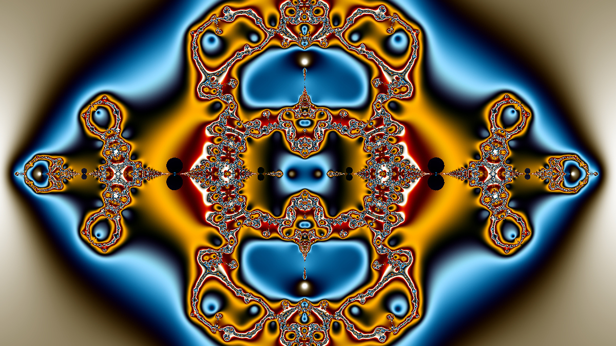 Secant Cosine | 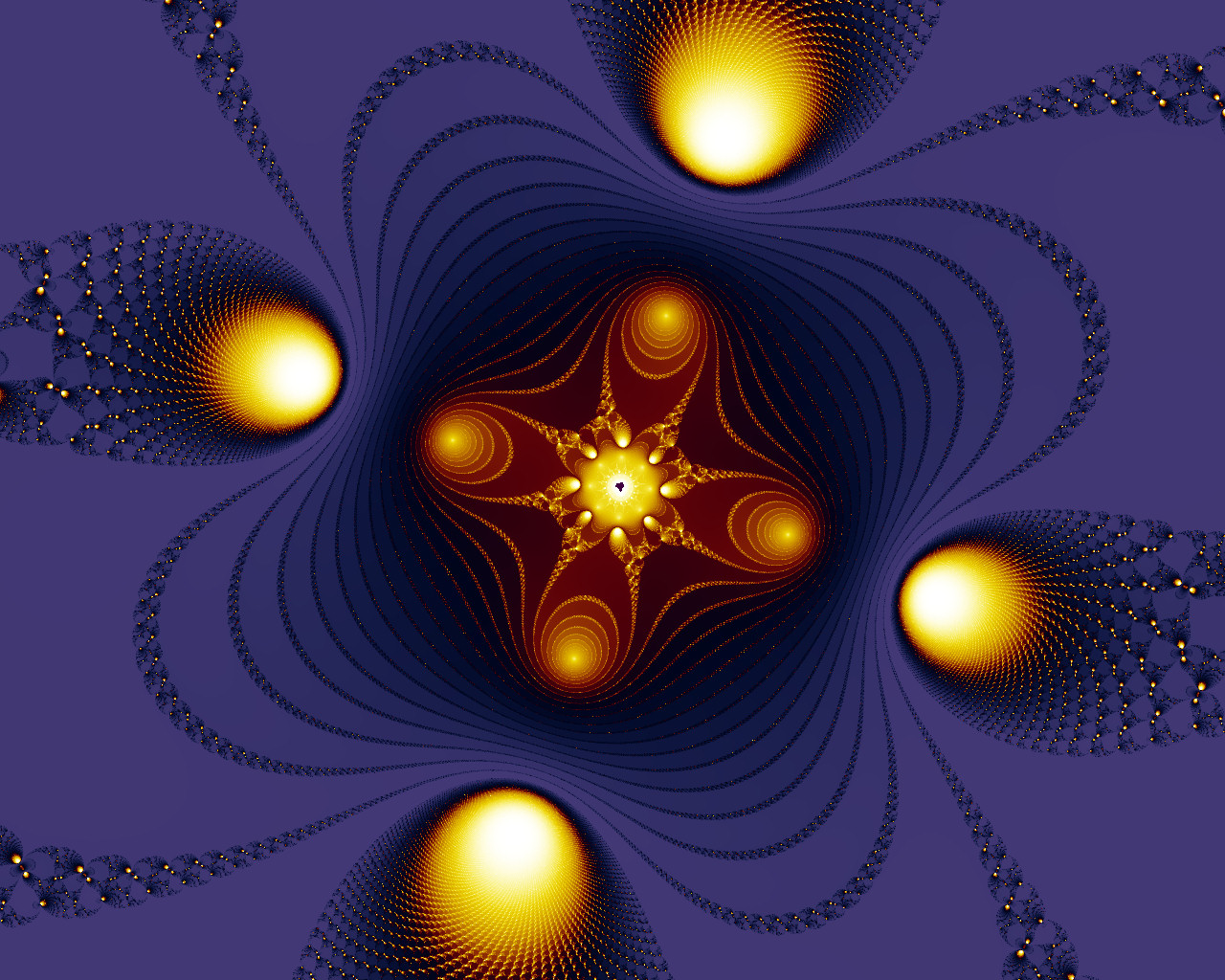 Four Kisses |
 |  |
    |
 |
  |
  |
   |
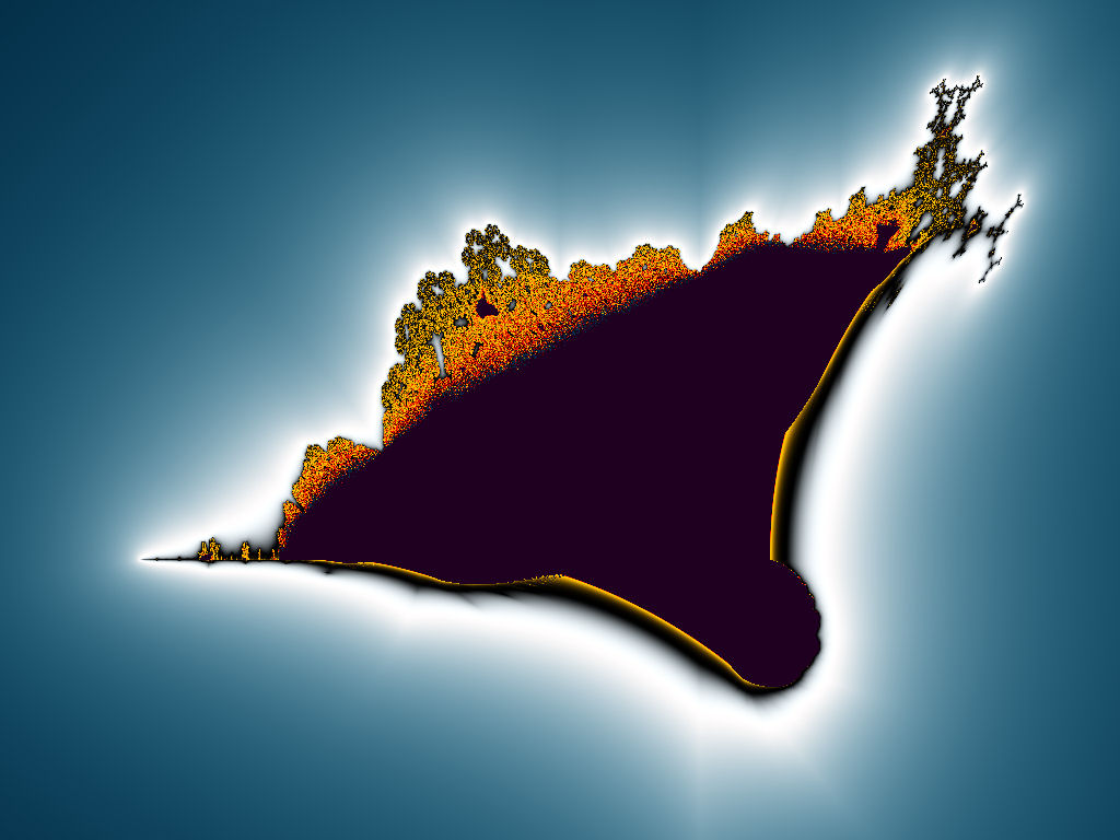
   A few very early, quick snapshots of the fractal that comes from the Henon map, illustrating some of its Julia sets, and one of the Mandelbrot-like sets for this function. |
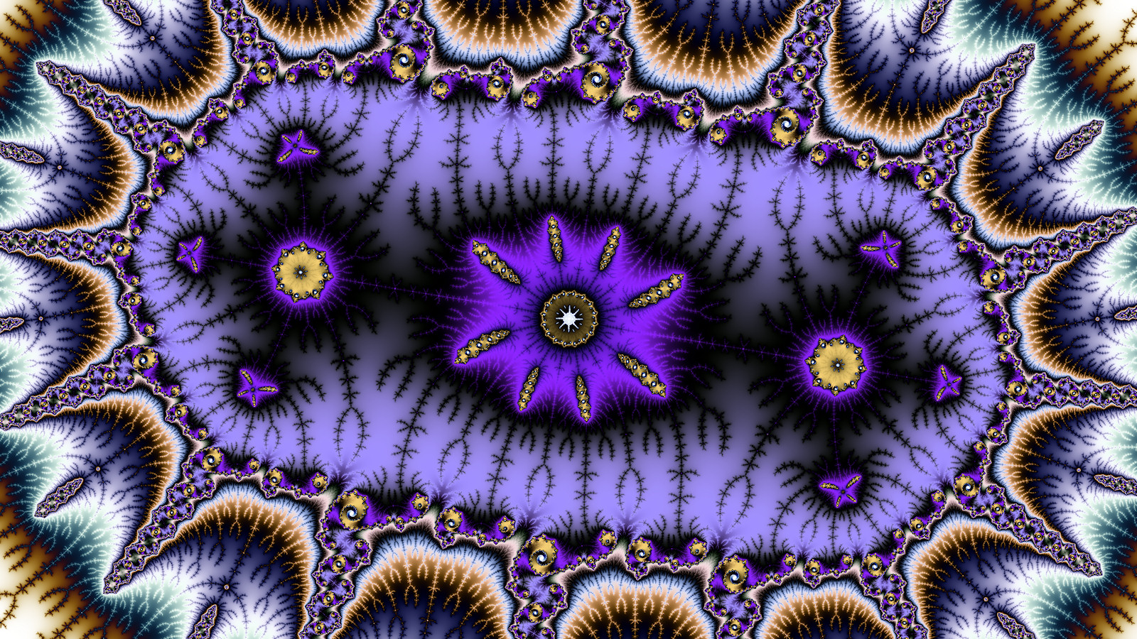
| High-Resolution Video Frame Captures | So far I have just made one, but more will be on the way. All the videos have tons of frames that would make great high-resolution still images, and I may start a project to render and upload a bunch of these. Each video page does have a few frame captures, but they are not typically rendered at ultra-high resolution or with aggressive anti-aliasing. This is from the animation GroupB, and is the 134th master image used for the frame interpolation. This image was rendered with 3x3 anti-aliasing (unlike the images used to make the video) for an ultra-high quality, noise-free final product.  Click on one of these download options: 1600x900 920KB High-resolution, moderate JPEG compression 2400x1350 5.04MB Ultra-resolution, very little JPEG compression |
Note on size and magnification: The sizes here (and on the Animations page) are the actual size of the smallest dimension of the image (usually vertically) in the complex number plane. Some programs describe image sizes by "magnification" which is usually related to the reciprocal of the image size. A size of, say, 1E-100 corresponds to a magnification of 1E+100. Some software uses the half-height of the image, so there may be an additional factor of two involved in conversion.
All content Copyright by Michael Condron. All rights reserved unless otherwise noted.
You may download, save, and print a single copy for personal use only.
Music by various sources used with permission.
Please refer to individual video file credits for details.
