hpdz.net
High-Precision Deep Zoom
Technical Info
Floating Point Arithmetic
The debacle of the bogus Magnet Fractal video finally drove me to launch a project I've been wanting to do for several years: get an arbitrary-precision floating point arithmetic library incorporated into the fractal software. The fixed-point arithmetic code has been working great for years, and it is very fast, but it has limitations that make it unsuitable for many types of fractals, especially those whose underlying function requires division. The artifacts in the Magnet Zoom video were due to overflows in the arithmetic that would never have happened with a good set of floating-point arithmetic routines.
This took a fair amount of work, but now HPDZ is cruising with a slick floating point arithmetic core that is pretty fast and very accurate.
Another big improvement, independent of the floating-point upgrade, is the development of an assembly-language binary division function. This new function is almost ten times faster than the previous division operation, which was based on Newton's method implemented with high-level C++ operations (easy to code, but highly inefficient). More on this below.
More information on the details of this follow below. Here are some links to the major topics on this page:
- Fixed-Point vs Floating Point
- Technical Details
- Core Division Function
- Division Core Speed
- Performance of C++ operators
- Bloopers
First is an introduction to fixed-point and floating-point numbering, with a few quick examples demonstrating the advantages and disadvantages of each system, and showing how a problem with the fixed-point system led to the bogus Magnet Fractal zoom video. After that is a more technical description of the details of the floating-point code, including a detailed explanation of the binary division function. Following are some measurements of the division core speed and the C++ operators. Finally, some fun images that came out when the code was not properly working.
Fixed-Point vs Floating-Point
Fixed-Point Representation of Numbers
In a fixed-point system, a certain fixed number of digits is assigned to represent the integer part of a number, and the rest of the digits are the fractional part. This allows numbers to have a very high precision, since a large number of digits can be included after the decimal point. This is what various numbers in a fixed-point system would look like with decimal numbers, using two digits for the integer and 6 digits for the fraction.
01.000000
00.500000
00.000001 (the smallest possible number)
99.999999 (the largest possible number)
Representing numbers like this has some big advantages, but it also has some drawbacks. The main advantage is that the decimal points are always aligned, so adding, subtracting, and comparing two numbers is quite easy -- just add digit-by-digit and you have the sum. The details are shown on the bignum arithmetic page.
The main disadvantage of this method is that the range of numbers that can be represented is limited. In this particular example, the largest number is slightly less than 100. If the application does not need numbers larger than 100, this may be perfectly acceptable. Indeed, the Mandelbrot set and many similar fractals can be drawn quite nicely with integer parts no greater than 100, and really it is possible to draw the set with numbers no larger than 4.
The other problem with this type of number system is that it is not necessarily closed under division. That means that there are many pairs of numbers, a and b, that are perfectly fine fixed-point numbers, but for which x = a / b is not representable. Here are some examples:
00.000060 / 80.000000 = 00.000000075 Too small
The first condition is an overflow: the result is too big to fit into the structure that represents the numbers. The second condition is an underflow: the result is too small to be represented. An undetected overflow is what caused the interesting, but bogus, structures in the Magnet Fractal zoom of October, 2010.
Of course, it's possible to specify that there be an equal number of digits to the left and right of the decimal point (four and four, for example, if we are considering 8-digit representations). This reduces the division problem, but does not eliminate it, and potentially wastes a lot of space, depending on the application. There is a better, more flexible way to represent numbers that will span a wide range of magnitudes, which is to allow the decimal point to "float".
Floating-Point Representation of Numbers
Floating point arithmetic, unlike the previous fixed-point arithmetic, represents numbers as a string of digits combined with an exponent. The exponent specifies where the decimal point goes, and the digits specify the value of the number. This is very much like scientific notation, where 10.0 is written as 1x101 and 1000 is 1x10³, etc. Here are some examples in a system with 8 digits of number and 2 digits of exponent (along with a +/- sign):
| 10000000 E+00 | 0.1 |
| 10000000 E+01 | 1.0 |
| 10000000 E-01 | 0.01 |
| 98765432 E+05 | 98765.432 |
| 10000000 E-99 | Smallest representable number |
| 99999999 E+99 | Largest representable number |
Note that I have chosen E00 to mean that the decimal point is immediately to the left of the first digit; this choice is arbitrary.
This system allows numbers of a much larger range to be represented, while maintaining the same number of significant digits across a wide span of magnitudes. This is a big advantage. Additionally, while it is still possible to find numbers for which a / b causes an overflow or underflow, this representation allows a much larger set of numbers to be divided (and multiplied) since the numbers can adjust their exponents to span larger magnitudes easily.
Floating-point arithmetic has many advantages, which is why all modern computer processors (even most graphics processors on video cards!) provide very powerful hardware support for arithmetic with numbers in this format, and a large volume of literature has been generated describing standards and analyzing performance of floating-point arithmetic. Probably the most commonly used format is what is described in the IEEE-754 specification, which is how all Intel and AMD processors internally work with floating-point numbers.
The disadvantage of representing numbers in a floating-point format is that addition is now very complicated. Since the decimal points are no longer aligned, the digits representing the numbers have to be shfited around internally before numbers can be added. For example, consider 10 + 0.005. These numbers are represented as
50000000E-02
Clearly we can't just add the digits as they are aligned here. We have to either shift right the digits of the number with the smaller exponent or shift left the digits of the number with the larger exponent. Let's shift right (this choice is arbitrary). The amount to shift is the difference between the exponents, which is 4:
+ 50000000
--------------
100050000000 -> 10005000E+02 = 10.005
Notice that there are extra 0's hanging off the right. In this particular example, these digits can just be ignored becasue they are 0, but in more realistic examples, they are used to round off the final result so it fits into the 8-digit space we have chosen to hold our numbers. Here is an example of an addition where rounding affects the final answer: consider 1.2345678 + 0.00012349876:
Shift, align, and add:
12345678
000012349876
------------
123469129876 -> 12346912(9876) -> 12346913
Rounding of floating-point numbers is actually a more complicated topic than you might think, and we will look at it again below.
Multiplication and division of floating-point numbers is essentially the same as the corresponding fixed-point operaitons, with the additional step of adding or subtracting the exponents.
A Hybrid Approach
The multi-precision fixed-point numbers are still used in the code, since they are perfectly fine for many purposes and are significantly faster than the multi-precision floating-point numbers. Coordinates and parameters are still represented as fixed-point numbers. Fractals that require division, such as the Magnet fractal and all fractals based on Newton's method (like the Nova fractal) have been rewritten to use floating-point numbers in the internal iteration loops.
Technical Details
The rest of this page will describe the technical details of implementation of the floating-point numbers, including issues related to rounding. The assembly-language binary division function will be described in some detail, and performance data will be presented.
Internal Representation of Numbers
Internally, the software represents numbers as an array of unsigned 32-bit integers, also called "double words" or DWORDs. The array always contains an even number of DWORDs. Sometimes, especially with the code now running in 64-bit mode, it is more convenient to think of them as an array of 64-bit integers, also called "quad words" or QWORDs. A single flag indicates the sign (positive or negative) of the number.
The "precision" of a number is the number of DWORDs it contains. I have stuck with this definition for the floating-point numbers as well, to keep the terminology simple. Precision increments in units of 2, since the underlying assembly language code has been working with 64-bit units for a long time, using either 64-bit general purpose instructions, or 64-bit SSE instructions.
Fixed-point numbers are represented as a single DWORD integer and an arbitrary number of DWORDs for the fractional part. A precision-4 fixed-point number uses 1 DWORD for integer and 3 DWORDs to hold 3x32=96 bits of fraction. A precision-8 fixed-point number will have 7x32=224 bits of fraction.
Floating-point numbers have an arbitrary number of DWORDs representing the significand (the digits of the number, also called "mantissa") and a signed 32-bit integer representing the exponent. At least half the 31-bit range of exponent values needs to be reserved for internal overflow detection, so the allowable range of exponents was chosen to be +/-0x20000000. The significand is stored as an unsigned value, and the sign of the number is held as a flag. The significand is normalized, with an explicit 1 in the most-significant bit always (unlike the IEEE754 format, which has an implicit 1).
Other states defined in the IEEE specification, like like NAN and INF (concepts from the IEEE-754 standard) are held in a separate flag field, rather than being represented by special values of the exponent or significand. Signed zero is supported, although I'm not sure I really need it right now. Denormalized numbers are kind of supported, but not completely. Right now, the type of underflow that leads to the need for a denorm is simply trapped as an exception. For drawing fractals, I'm not sure denorm support is a high priority.
Floating Point Addition and Subtraction
This essentially follows Knuth's Algorithm A in The Art of Computer Programming, Vol 2, page 200. The main difference is that I keep one full extra 64-bit guard "digit" in the intermediate step following the shifting to align the radix points. The smaller number is shifted into a temporary buffer with this extra QWORD, and the resulting least-significant 64 bits of the sum are used to effect the rounding operation, which is described in more detail below.
Rounding and normalizing are kind of complicated. After the aligned values are added, there may be a carry out of the most-significant place, or, in the case of subtraction, the result may not be normalized if some of the most-significant bits cancel out. Knuth's Algorithm N handles all this. I implemented essentially the same concepts like this:
Shift significand right one bit
Adjust exponent (+1)
If (exponent overflow)
throw (Overflow Exception)
Else
pos = position of most significant nonzero bit
If (pos > 0)
Shift significand left (pos) places
Adjust exponent (-pos)
If (exponent underflow)
throw (Underflow Exception)
Else If (all bits are 0)
Set exponent = 0
Round significand (unnecessary if zero)
If (overflow after rounding)
Shift significand right one bit
Adjust exponent (+1)
If (exponent overflow)
throw (Overflow Exception)
Other bookkeeping matters to be attended to include handling inputs of NAN, INF, etc., and how to handle inputs of different precisions. I followed the IEEE754 rules for NAN and INF. If the inputs have different precisions, the intermediate calculations are carried out in the higher precision and the returned value is in the higher precision.
The function to actually add the digits is assembly-language code from the fixed-point system. Left and right shifts are also coded in assembly language, as is the function to locate the most-significant nonzero bit. The rest of the addition function that handles all the decision-making is in C.
Multiplication and Division
These operations are much easier than addition -- provided you already have code available to perform the calculations on the significand's digits. The significands are simply treated the same as fixed-point numbers, except that there is no overflow condition if there's a carry beyond the most-significant place. If a carry is generated, the product is simply shifted right one place and the exponent is adjusted.
Multiplication code is already in place from the fixed-point numbers, and it is applied to the floating-point numbers with only a small modification to handle the lack of overflow. The multiplication code is all assembly-language, wtih highly optimized specialized functions for small 2x2 and 4x4 blocks of products. A 2x2 block is really a single 64-bit multiplication, and a 4x4 block is 4 64-bit multiplications with some adds. In the current 64-bit version of the software, the 64-bit general purpose instructions are used, rather than the SSE instructions. These small code blocks for 2x2 and 4x4 are combined to form unrolled code for multiplications up to 16x16. Beyond precision 16, a loop is used.
As part of the development of the floating-point number code, I chose to write an assembly-language division function, something I've been wanting to do for several years. More on that below.
Rounding
Rounding is a surprisingly subtle and complicated operation. The idea is that since numbers in the computer are represented as discrete quantities (whether fixed-point or floating-point) a decision has to be made how to handle results of calculations that fall between two numbers that can be represented exactly.
In the 8-digit addition example above, the result of 1.2345678 + 0.00012349876 is exactly 1.23469129876. But that number has 12 digits, which is too many to fit into our 8-digit number system. Rounding is the process of choosing one of the two exactly representable values nearest to such a result as the final answer. There are many ways to do this, all spelled out in detail in the IEEE specification, like round toward zero (this is the same as simply truncating the extra digits), round toward -infinity or +infinity (these differ when you think about how to round negative numbers), etc.
Most rounding methods are not recommended for common use, but they all have specific specialized applications. The one that generally makes the most sense is round to nearest. That means that we choose the representable number that is closest to our exact result. Most of the time, that choice is easy, as in the above example, where the extra digits are 9876: we round the least-significant digit up one value, from 2 to 3, and the final result is 1.2346913. If, say, the final result had been 1.23469124321, we'd round down, to 1.2346912.
Round to nearest is better than simply truncating the result, chopping off the extra digits, because it does the best job of preserving the little bit of information those extra few digits contain. But what do you do when a result is exactly haflway between two representable numbers? Consider 1.23469125000. Should this be 1.2346912 or 1.2346913? The approach commonly taught in elementary school is to round the halfway cases up, and that's what many of us do in ordinary life when we're rounding things off. It seems to make intuitive sense, since 0,1,2,3,4 are five values that get rounded down, and 5,6,7,8,9 are five values that get rounded up. But that is not really the right way to look at the situation. Rather, consider that 0.5000... is exactly halfway between 0.0 and 1.0, so there's no way to favor one over the other.
Why not just round 0.5 to 1.0? Doing so introduces a subtle bias in the way the imprecision of the calculations is propagated. It slightly favors rounding things up, and over time, when many calculations are done and rounded with this bias, numbers can artifactually drift upward.
The solution to this problem is to round 0.5 in such a way that there is no net bias, sometimes rounding it up, and sometimes rounding it down. Several ways to do this have been devised, including simply randomly choosing a direction whenever this comes up. While choosing a random direction will work, what is usually done in computer arithmetic is to round to the nearest even digit, or to the nearest odd digit. This is illustrated in the table below, which demonstrates round-to-even:
| Exact Value | Rounds to | Comment |
| 1.23456705000 | 1.2345670 | Rounded DOWN |
| 1.23456715000 | 1.2345672 | Rounded UP |
| 1.23456725000 | 1.2345672 | Rounded DOWN |
| 1.23456735000 | 1.2345674 | Rounded UP |
| 1.23456745000 | 1.2345674 | Rounded DOWN |
| 1.23456755000 | 1.2345676 | Rounded UP |
| 1.23456765000 | 1.2345676 | Rounded DOWN |
| 1.23456775000 | 1.2345678 | Rounded UP |
| 1.23456785000 | 1.2345678 | Rounded DOWN |
| 1.23456795000 | 1.2345680 | Rounded UP |
In every case, the magnitude of the lost digits is 0.00000005, so rounding in this manner does not magnify the loss of information. But the sign of the error is evenly balanced between up and down, so in the long term, this kind of error will have no net bias (assuming positive and negative numbers occur with equal frequency).
How often does this matter? From the example I have chosen here, with 4 extra digits, you might think that the value 5000 in the last four digits occurs only very rarely. But actually this situation arises quite often. Consider, in decimal, what happens when you add two numbers whose exponents differ by 1. The extended result will have a 5 at the end 1/10th of the time! In binary, for numbers with exponents differing by 1, the exactly-in-between case arsies half the time (when there's a 1 in the LSB of the smaller number). If the exponents differ by 2, it arises 1/4 of the time, for a difference of 3, 1/8 of the time, etc. So this is by no means a rare event, and handling it correctly is very important.
Core Division Function
Background
The fixed-point numbers initially had no division at all. The first approach I took to implementing division for them was to do a binary search to find the reciprocal of the divisor.
Later I used the approach based on the Newton-Raphson method for solving equations: Let f(x) = 1/x - v. That function is zero when x=1/v, so if we can find the value of x where f(x) is zero, then we have 1/v. That can then be multiplied by u to get u/v. The Newton-Raphson method works very well. It can be calculated with only multiplications and add/subtract, and it converges pretty quickly. I implemented this in C++, which was quite easy, but was also quite slow.
Binary Division
The formidable Algorithm D on page 257 of Knuth's The Art of Computer Programming, Vol 2, forms the basis of this function. For numbers formed from a small number of digits, and given a fast way to divide a 2-digit number by a 1-digit number, this is the most efficient algorithm I am aware of. The CPU DIV instruction can divide a 128-bit number by a 64-bit number, giving a 64-bit quotient and remainder, and that is the basic unit of action in this process. A "digit" here refers to a 64-bit quantity, two DWORDs from the significand of a high-precision floating-point number.
There is no quick way to summarize how Algorithm D works. It is complicated, and the notation needed to discuss it is very tedious. In essence, it resembles manual long division, but it is adjusted a bit to be better suited to programming on a computer.
If you are considering writing code to implement Algorithm D, reading the description of the method is not sufficient. Part of the mission of this web site is to serve as a resource for learning some useful computer science and math, so we should emphasize that if you want to understand this algorithm, you have to run it on paper with a variety of test conditions, and also read the MIX implementation to see some subtle tricks.
The main steps are as follows, adjusted to better represent the situation of dividing two numbers of equal size, as we have here.
To obtain the base-b (my code uses 64-bit digits, so b is 2^64) n-digit quotient q = u / v, where u=(u1,...,un) and v=(v1,...,vn), and assuming u and v are both normalized:
- Copy u into a buffer of size 2n+1, padding with n zeros to the right and one zero to the left. This creates a new u=(u0,...,u2n) with u0=0 and un+1...u2n=0: u=(0,u1,...,un,0,...0).
- Initialize a loop counter j = 0. This will label the quotient digits, qj, and the dividend digits, uj.
-
Obtain guess g at quotient digit qj.
If v1 = uj, the guess is g = b-1. Otherwise, g is the quotient of the two-digit number formed by uj shifted left one digit, plus uj+1. Keep the remainder of this division and call it r.
There's a good bit of theory behind why the particular approach to this guess described here works, and the theory is delivered in Theorem A and Theorem B on pages 256 and 257. The guess is very often exactly right, and nearly always just 1 too big. Rarely, it is 2 too big. -
Test whether v2g > rb + uj+2. If it is, decrease g
by 1, add v1 to r, and test again.
Note that this test is of two 128-bit numbers. This can all be done with single-digit comparisons and some clever register usage. The iteration here does not require any more multiplication, just single-digit subtraction and addition. The example MIX code on page 259 shows how to do this. -
Multiply g * v and subtract from uj...uj+n. Note that
this can be done in-place and in a single loop on the buffer that was
created in step 1, although it's tricky to manage the borrows. The
alignment of the subtraction is such that the low-order digit of gvn
is subtracted from uj+n. The high-order digit of gv1,
plus any borrow from the right, is subtracted from uj-1.
This subtraction may generate a borrow from uj-1. If so, then the guess g is too big. Decrement it by 1 and add v back into u at the same position where we just subtracted it. - Save g into the array for u created in step 1 at position j.
- Increment j and go back to step 3 if j <= n.
The temporary array that was filled wtih u in step 1 will now hold q=(q1,...,qn) along with one digit qn+1 of remainder and a possible overflow digit q0. The overflow q0 will be nonzero if u > v, which means the quotient is goign to be greater than 1. In any event, round and normalize etc. and adjust the exponents as needed.
That's it.
Accuracy
Simulation with nearly a billion runs of random test data at all precisions, and also with data contrived to test corner cases, shows that this operation:
x = (a / b) * b - a
gives identically 0 about 89% of the time and gives 1ULP of error the remaining 11% of the time. (1 ULP is a "unit in the last place" which is +/- 1 least-significant bit of error).
Division Core Speed
Accurately measuring the speed of an assembly-language subroutine is tricky, since the overhead of the typical ways of measuring speeds in C can easily dominate the measurement. Furthermore, the speed of the code in actual time is dependent on processor clock speed. A more objective and constant measure of the efficiency of a piece of code like this is how many clock cycles it takes to execute. For a multi-precision arithmetic operation, it is also helpful to see how the number of clock cycles varies with the size of the number, as the precision increases.
To do this properly, the time-stamp counter register in the CPU has to be accessed with the RDTSC instruction. This 64-bit counter is incremented every clock cycle, so by reading it at the start and end of a short body of code, we can see how many clock cycles that code took to run.
This is a little bit complicated because RDTSC is not a serializing instruction, meaning that it does not necessarily wait until all previous instructions have executed before reading the counter. This is a hassle, but it can be worked around by inserting a serializing instruction like CPUID before it. CPUID, unfortunately, takes dozens to hundreds of clock cycles to execute, so a lot of test points have to be inserted into the code to measure the time the code is running and also measure how long the CPUID instructions are taking.
The table and graphs below show the results of these measurements, which have beeen done as carefully as I can figure out how to do them. These are averages over 10 million calls to the division core function, subtracting off time for setting up the stack frame and copying the dividend to the temporary buffer.
The N here that is used to scale the clock cycles is the number of 64-bit DWORDs in the number size, which is half the "precision" value in the tables (that is, a precision 8 number is made of 4 64-bit QWORDs, so N=4). Each iteration of the division algorithm determines a 64-bit "digit" of the quotient, so this N is the appropriate scale factor to evaluate the efficiency of each iteration.
| Precision | Clock Cycles | Cycles/N | Cycles/N2 |
|---|---|---|---|
| 4 | 190 | 95.0 | 47.5 |
| 6 | 335 | 113 | 37.6 |
| 8 | 511 | 128 | 31.9 |
| 12 | 912 | 152 | 25.3 |
| 16 | 1408 | 176 | 22.0 |
| 24 | 2657 | 221 | 18.5 |
| 32 | 4255 | 266 | 16.6 |
| Precision | Clock Cycles | Cycles/N | Cycles/N2 |
|---|---|---|---|
| 4 | 151 | 75.5 | 37.8 |
| 6 | 338 | 113 | 37.6 |
| 8 | 442 | 111 | 27.6 |
| 12 | 912 | 152 | 25.3 |
| 16 | 1480 | 185 | 23.1 |
| 24 | 3073 | 256 | 21.3 |
| 32 | 5183 | 324 | 20.3 |
Performance of High-Level C++ operators
The tables and graphs below show the relative speeds of the fixed-point and floating point systems. These are measured at the high-level C++ operators and therefore include all the associated overhead of creating temps and such. These are the most realistic numbers to measure how fast the code can be expected to calculate complicated fractal formulas.
These are all measured on the 4.0 GHz Core i7 980X system.
The full spread of precisions currently supported ranges from 4 to 34 in increments of 2. I have selected a few representative values here to keep the table smaller.
Addition
| Precision | Fixed-point | Floating-point | Ratio of speeds |
|---|---|---|---|
| 4 | 40.5 | 15.1 | .37 |
| 6 | 35.1 | 13.4 | .38 |
| 8 | 30.8 | 12.1 | .39 |
| 12 | 24.6 | 10.0 | .41 |
| 16 | 21.0 | 8.67 | .41 |
| 24 | 15.9 | 6.75 | .42 |
| 32 | 12.8 | 5.47 | .43 |
Addition with the floating-point numbers is about 40% as fast as with fixed-point numbers. That's not bad considering all the shifting around that has to be done.
Multiplication
| Precision | Fixed-point | Floating-point | Ratio of speeds |
|---|---|---|---|
| 4 | 33.4 | 19.7 | .59 |
| 6 | 22.0 | 14.3 | .65 |
| 8 | 19.4 | 12.4 | .64 |
| 12 | 13.0 | 8.58 | .66 |
| 16 | 8.81 | 6.42 | .73 |
| 18 | 4.84 | 3.79 | .78 |
| 24 | 3.13 | 2.64 | .84 |
| 32 | 2.03 | 1.79 | .87 |
Multiplication is similar in speed between the two number systems, which is not surprising since they both use the same underlying code. As the number of digits increases, the small additional overhead of the floating-point system has less impact on the speed difference, and 32-digit (1024-bit) multiplication runs at nearly the same speed. There is an abrupt change in speed from precision 16 (512 bits) to precision 18 because the optimized unrolled multiplication code only goes to precision 16; beyond that, a loop is used.
Division
| Precision | Fixed-point | Floating-point | Ratio of speeds |
|---|---|---|---|
| 4 | 1.67 | 8.49 | 5.08 |
| 6 | 1.06 | 6.31 | 5.95 |
| 8 | 0.977 | 4.86 | 4.97 |
| 12 | 0.611 | 3.08 | 5.04 |
| 16 | 0.480 | 2.14 | 4.46 |
| 18 | 0.263 | 1.82 | 6.92 |
| 24 | 0.186 | 1.20 | 6.45 |
| 32 | 0.131 | 0.765 | 5.84 |
Division is significantly faster in the floating-point system because it is using the high-speed assembly language core, while the fixed-point numbers are still using an implementation of Newton-Raphson convergence in high-level C++.
Relative Times
Finally, it is useful to know what the time of an operation is in in terms of how long it takes to do that operation relative to the time it takes to do addition at the same precision.
| Precision | Multiplication | Division |
|---|---|---|
| 4 | .77 | 1.78 |
| 6 | .94 | 2.14 |
| 8 | .98 | 2.49 |
| 12 | 1.17 | 3.25 |
| 16 | 1.35 | 4.05 |
| 18 | 2.14 | 4.45 |
| 24 | 2.56 | 5.63 |
| 32 | 3.06 | 7.15 |
At lower precisions, multiplication is actually slightly faster than addition! That is because of all the additional overhead associated with shifting to align radix points in the addition code. Overall, multiplications are only slightly more expensive than additions in this system. A division costs anywhere from about 2 to 4 additions for the range of precision where most fractal zooms are made (precision 4 to 16).
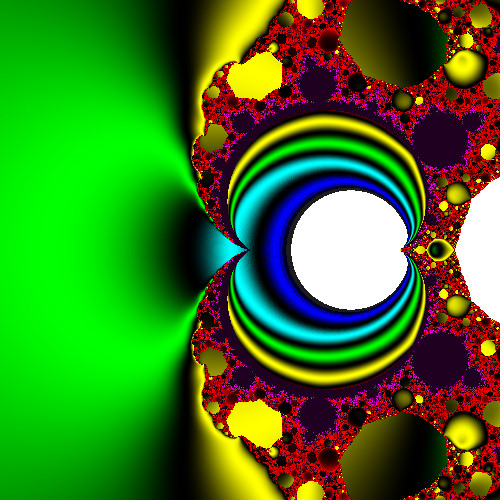
Bloopers
Nothing as complex as this can be expected to go off smoothly every step of the way. Here are some of the earliest images generated with the floating-point arithmetic code, showing that some debugging still needed to be done.
As always, click on a thumbnail to get a larger image.

The above image was the first attempt at drawing the magnet fractal with the floating point code. Clearly some additional work was needed. I thought maybe the formula was too complex, so I tried something simpler, which yielded the next image.
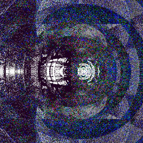
This was using Newton-Raphson division. The machine code division came later.

This is the first Newton fractal with the new floating point code. This is obviously not working right. Also, you can see how most arithmetic errors give images that are just total garbage, not the beautiful, clean tricorn shape that showed up in the bogus magnet fractal zoom.
It turned out that the problem was in the rounding step in the multiplication function. Once in a great while (i.e. far more often than you'd expect) the rounding action causes an overflow, which means the whole result has to be shifted right 1 bit and the exponent has to be adjusted. This was handled properly in the addition function but not in the multiplication function.
After that problem was fixed, the following two lovely images were generated.

Finally, below is the result of the first attempt to draw the magnet fractal with the binary machine-code division function. The problem here was in the wickedly complicated multiply-and-subtract in-place operation. It took 5 tries to finally get this right.
All content Copyright by Michael Condron. All rights reserved unless otherwise noted.
You may download, save, and print a single copy for personal use only.
Music by various sources used with permission.
Please refer to individual video file credits for details.
